The main plotting function for one or several Gviz tracks.

plotTracks is the main interface when plotting single track objects, or lists of tracks linked together across the same genomic coordinates. Essentially, the resulting plots are very similar to the graphical output of the UCSC Genome Browser, except for all of the interactivity.

plotTracks(
  trackList,
  from = NULL,
  to = NULL,
  ...,
  sizes = NULL,
  panel.only = FALSE,
  extend.right = 0,
  extend.left = 0,
  title.width = NULL,
  add = FALSE,
  main,
  cex.main = 2,
  fontface.main = 2,
  col.main = "black",
  margin = 6,
  chromosome = NULL,
  innerMargin = 3
)

Arguments

trackList: A list of Gviz track objects, all inheriting from class GdObject. The tracks will all be drawn to the same genomic coordinates, either as defined by the from and to arguments if supplied, or by the maximum range across all individual items in the list.
from, to: Character scalar, giving the range of genomic coordinates to draw the tracks in. Note that to cannot be larger than from. If NULL, the plotting ranges are derived from the individual tracks. See extend.left and extend.right below for the definition of the final plotting ranges.
...: Additional arguments which are all interpreted as display parameters to tweak the appearance of the plot. These parameters are global, meaning that they will be used for all tracks in the list where they actually make sense, and they override the track-internal settings. See settings for details on display parameters.
sizes: A numeric vector of relative vertical sizes for the individual tracks of length equal to the number of tracks in trackList, or NULL to auto-detect the most appropriate vertical size proportions.
panel.only: Logical flag, causing the tracks to be plotted as lattice-like panel functions without resetting the plotting canvas and omitting the title pane. This allows to embed tracks into a trellis layout. Usually the function is called for a single track only when panel.only==TRUE.
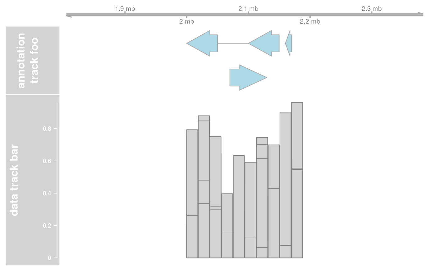
extend.right, extend.left: Numeric scalar, extend the plotting range to the right or to the left by a fixed number of bases. The final plotting range is defined as from-extend.left to to+extend.right.
title.width: A expansion factor for the width of the title panels. This can be used to make more space, e.g. to accommodate for more detailed data axes. The default is to use as much space as needed to fit all the annotation text.
add: Logical flag, add the plot to an existing plotting canvas without re-initialising.
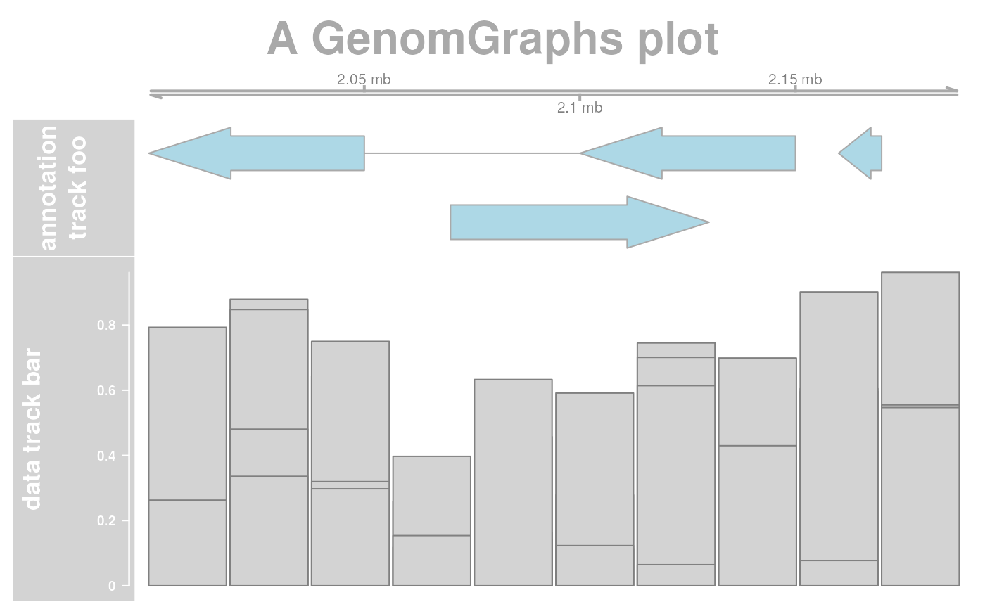
main: Character scalar, the plots main header.
cex.main, fontface.main, col.main: The fontface, color and expansion factor settings for the main header.
margin: The margin width to add to the plot in pixels.
chromosome: Set the chromosome for all the tracks in the track list.
innerMargin: The inner margin width to add to the plot in pixels.

Value

A list of Gviz tracks, each one augmented by the computed image map coordinates in the imageMap slot, along with the additional ImageMap

object titles containing information about the title panels.

Details

Gviz tracks are plotted in a vertically stacked layout. Each track panel is split up into a title section containing the track name, as well as an optional axis for tracks containing numeric data, and a data section showing the actual data along genomic coordinates. In that sense, the output is very similar to the UCSC Genome Browser.

The layout of the individual tracks is highly customizable though so called "display parameters". See settings for details.

While plotting a track, the software automatically computes HTML image map coordinates based on the current graphics device. These coordinates as well as the associated annotation information can later be used to embed images of the plots in semi-interactive HTML pages. See ImageMap for details.

Author

Florian Hahne

Examples

## Create some tracks to plot
st <- c(2000000, 2070000, 2100000, 2160000)
ed <- c(2050000, 2130000, 2150000, 2170000)
str <- c("-", "+", "-", "-")
gr <- c("Group1", "Group2", "Group1", "Group3")
annTrack <- AnnotationTrack(
    start = st, end = ed, strand = str, chromosome = 7,
    genome = "hg19", feature = "test", group = gr,
    id = paste("annTrack item", 1:4),
    name = "annotation track foo",
    stacking = "squish"
)

ax <- GenomeAxisTrack()

dt <- DataTrack(
    start = seq(min(st), max(ed), len = 10), width = 18000,
    data = matrix(runif(40), nrow = 4), genome = "hg19", chromosome = 7,
    type = "histogram", name = "data track bar"
)
# \dontshow{
## For some annoying reason the postscript device does not know about
## the sans font
if (!interactive()) {
    font <- ps.options()$family
    displayPars(annTrack) <- list(fontfamily = font, fontfamily.title = font)
    displayPars(ax) <- list(fontfamily = font, fontfamily.title = font)
    displayPars(dt) <- list(fontfamily = font, fontfamily.title = font)
}
# }


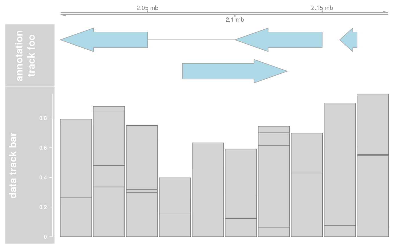
## Now plot the tracks
res <- plotTracks(list(ax, annTrack, dt))


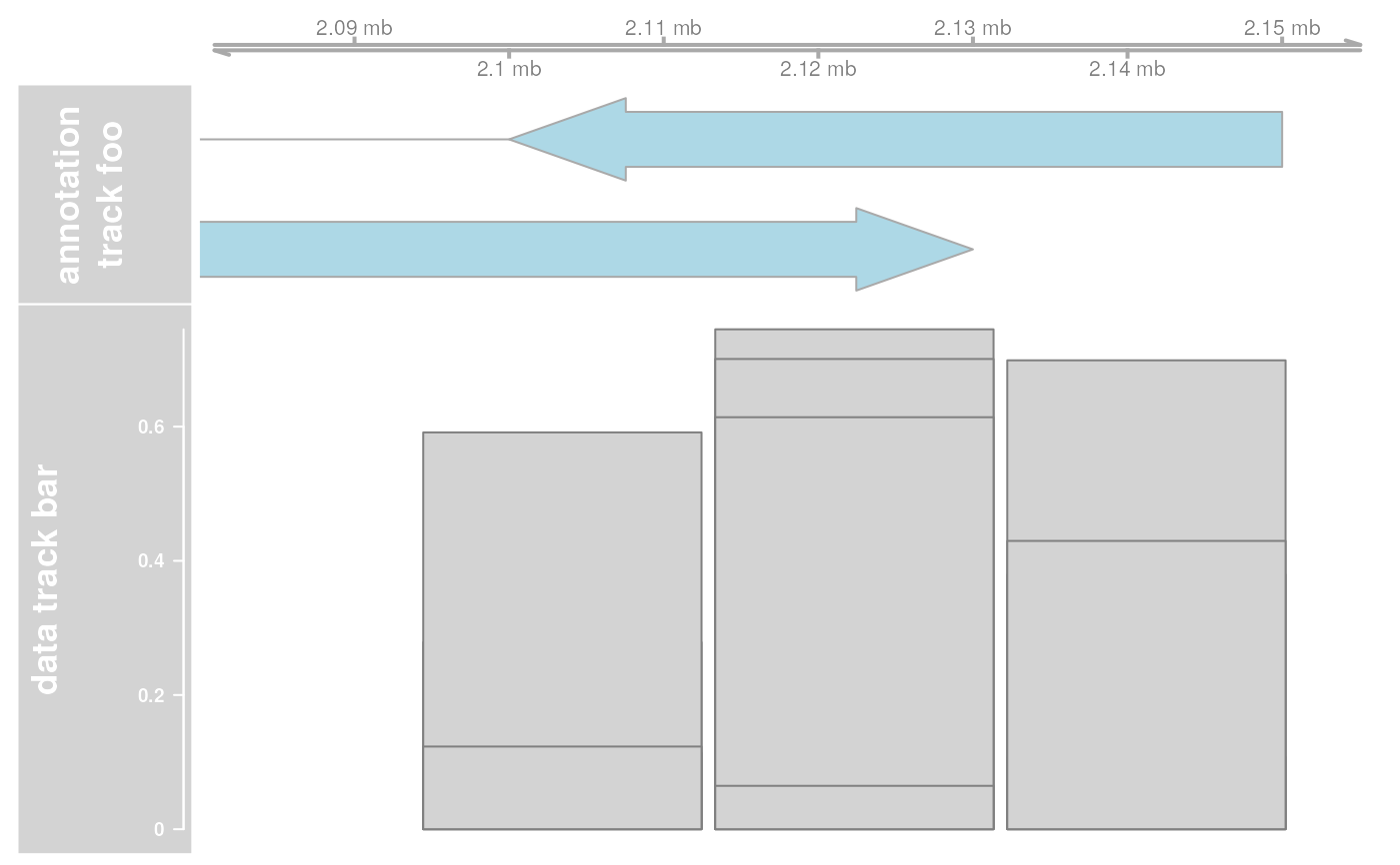
## Plot only a subrange
res <- plotTracks(list(ax, annTrack, dt), from = 2080000, to = 2156000)


## Extend plotting ranges
res <- plotTracks(list(ax, annTrack, dt), extend.left = 200000, extend.right = 200000)


## Add a header
res <- plotTracks(list(ax, annTrack, dt),
    main = "A GenomGraphs plot",
    col.main = "darkgray"
)


## Change vertical size and title width
res <- plotTracks(list(ax, annTrack, dt), sizes = c(1, 1, 5))


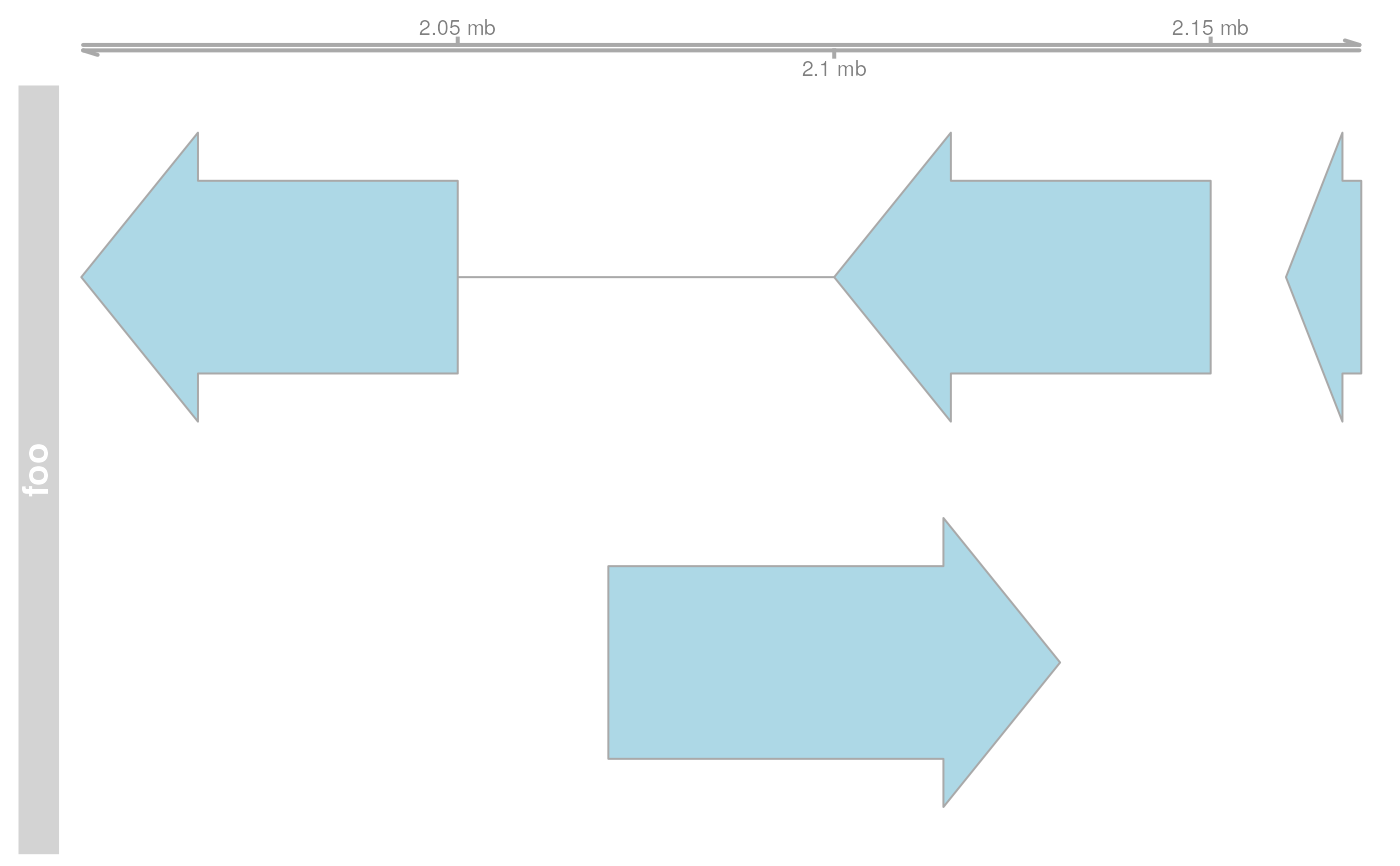
names(annTrack) <- "foo"
res <- plotTracks(list(ax, annTrack), title.width = 0.6)


## Adding and lattice like plots
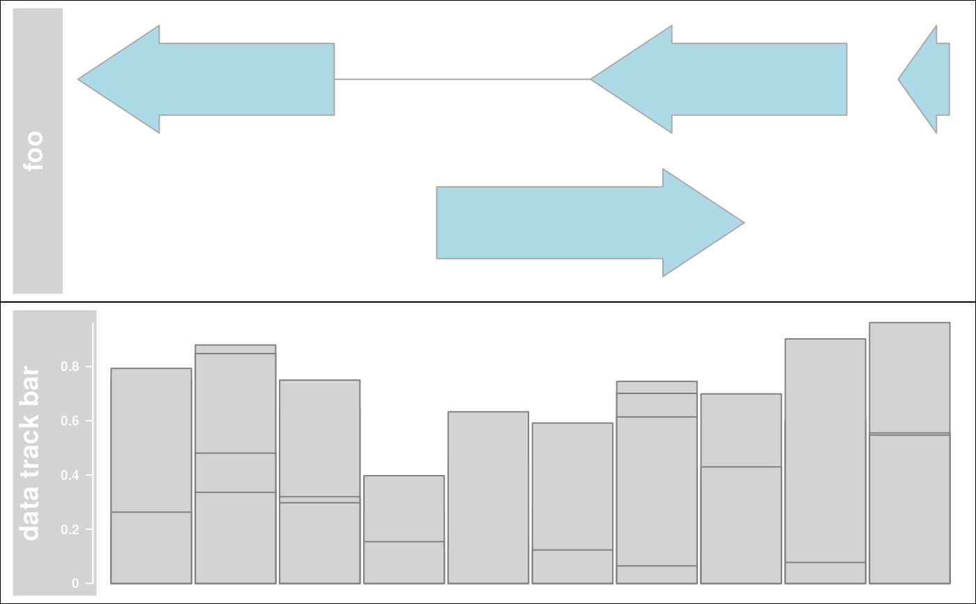
library(grid)
grid.newpage()
pushViewport(viewport(height = 0.5, y = 1, just = "top"))
grid.rect()
plotTracks(annTrack, add = TRUE)
popViewport(1)
pushViewport(viewport(height = 0.5, y = 0, just = "bottom"))
grid.rect()
plotTracks(dt, add = TRUE)
popViewport(1)

if (FALSE) {
library(lattice)
myPanel <- function(x, ...) {
    plotTracks(annTrack,
        panel.only = TRUE,
        from = min(x), to = max(x), shape = "box"
    )
}
a <- seq(1900000, 2250000, len = 40)
xyplot(b ~ a | c, data.frame(a = a, b = 1, c = cut(a, 4)),
    panel = myPanel,
    scales = list(x = "free")
)
}